1. Basic Concepts of Repeated Measures:
In this basic setup of a completely randomized design with repeated measures, there are two
factors, treatments and time.
Treatment is called the between-subjects factor because levels of treatment can change only between subjects; all measurements on the same subject will represent the same treatment.
Time is called a within-subjects factor because different measurements on the same subject are taken at different times.
In repeated measures experiments, interest centers on (1) how treatment means differ, (2) how treatment means change over time, and (3) how differences between treatment means change over time.
2. Four-step procedure for mixed model analysis:
Step 1: Model the mean structure, usually by specification of the fixed effects.
Step 2: Specify the covariance structure, between subjects as well as within subjects.
Step 3: Fit the mean model accounting for the covariance structure.
Step 4: Make statistical inference based on the results of step 3.
3. A Statistical Model for Repeated Measures:
Let Yijk denote the measurement at time k on the jth subject assigned to treatment i.
A statistical model for repeated measures data is
Yijk = μ + αi + γk + (αγ)ik + eijk
where
μ + αi + γk + (αγ)ik is the mean for treatment i at time k, containing effects for treatment, time, and treatment × time interaction.
eijk is the random error associated with the measurement at time k on the jth subject that is assigned to treatment i. The distinguishing feature of a repeated measures model is the variance and covariance structure of the errors, eijk.
we assume that errors for different subjects are independent, giving
Cov[eijk, ei'j'l] = 0 if either i ≠ i' or j ≠ j' (5.2)
since measurement on the same subject are over a time course, they may have different variances, and correlations between pairs of measurements may depend on the length of the time interval between the measurements. Therefore, in the most general setting, we only assume
Var[eijk] = σk2 and Cov[eijk, eijk'] = σkk' (5.3)
In some situations, it is advantageous to include a between-subjects random effect to give the model
Yijk = μ + αi + bij + γk + (αγ)ik + εijk (5.4)
where bij is a random effect for subject j assigned to treatment i, and εijk is an error with covariance matrix R with a parametric structure. The covariance matrix of Yij = [Yij1,…,Yijt]' becomes
Σ = Var[Yij] = σb2*J + R (5.5)
where J is a matrix of ones. Equation (5.5) shows the two aspects of covariance between measures on the same subject. The part σb2*J represents the covariance due to the fact that the measures are on the same subject, and R represents the contribution to the covariance due to the proximity of the measurements.
4. Using the REPEATED statement in PROC MIXED
The basic syntax of the REPEATED statement is as follows:
REPEATED variable name of repeated measures factor /
subject=combinations of variable names
defining sets of repeated measures
type=name of covariance structure;
Example:
HOUR is the repeated measures factor. The sets of repeated measures correspond to the individual patients. In the first illustration, no particular structure is imposed; that is, the covariance is “unstructured.” The PROC MIXED statements to fit the fixed effects of DRUG, HOUR, and DRUG × HOUR interaction, with unstructured covariance matrix Σ for each patient, are as follows:
proc mixed data=xxx;
class drug patient hour;
model fev1=drug hour drug*hour;
repeated hour / subject=patient(drug) type=un r rcorr;
run;
The REPEATED statement is used to define covariance matrix of the data vector conditional on
random effects, Var[Y|u] = R.
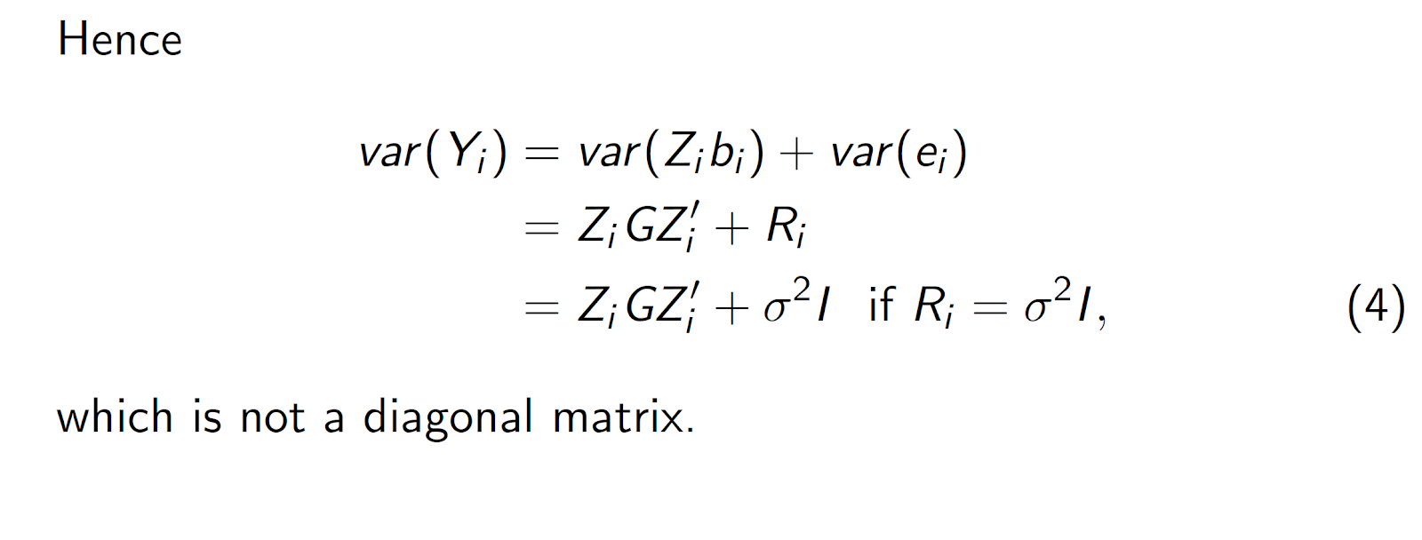
Recall that in the mixed model Y = Xβ + Zu + e, the random effects u have covariance matrix G and the errors e have covariance matrix R. Consequently, the variances of the conditional and marginal distributions are Var[Y|u] = R and Var[Y] =ZGZ' + R, respectively. (We frequently denote the marginal variance as V.) In a model without random effects (u = 0), the marginal and conditional variances are identical.
In this context, we use Σ to denote that portion of R that corresponds to an individual subject.
The important elements of the REPEATED statement are as follows:
1. The effect listed before the option slash (/). Here, HOUR is listed as this effect. The levels of the effect define the rows and columns of the matrix Σ in equation (5.4).
2. The SUBJECT= effect defines the effect whose levels identify observations belonging to the same subject. In the example, all observations that share the same levels of the PATIENT(DRUG) effect represent a single subject. Observations from different subjects are independent.
3. The TYPE= option determines the covariance structure in Σ.
4. The R option requests that PROC MIXED display the estimate of the R matrix (more precisely, the Σ matrix for the first subject).
5. The RCORR option requests the correlation matrix, which is obtained by computing correlations from the elements of the R matrix (a covariance matrix).
Mixed Model Analysis of Repeated Measures Using the REPEATED
Statement: Estimated Covariance Matrix—Unstructured
---SAS outputs for RCORR:
Mixed Model Analysis of Repeated Measures Using the REPEATED Statement: Estimated Correlation Matrix—Unstructured
Interpretation : You can see the decreasing trend in correlation with increasing lag.
The mixed procedure uses the REML method (Patterson and Thompson 1971) by default. This
method obtains estimates of covariance parameters by minimizing the likelihood of residuals from fitting
the fixed effects portion of the model.
---SAS outputs for Goodness of fit statistics:
Mixed Model Analysis of Repeated Measures Using the REPEATED Statement: Fit Statistics—Unstructured
Interpretation: The smaller AIC or BIC values, the better.
---SAS outputs
Mixed Model Analysis of Repeated Measures Using the REPEATED Statement: Null Model Likelihood Ratio Test—Unstructured
The “Null Model Likelihood Ratio Test” is a likelihood ratio test of whether the model with the specified covariance fits better than a model with errors—that is, with Σ =σ2*I. The p-value<.0001 shows that the iid N(0,σ2*I) model is clearly inadequate.
5. For a given linear model, how can we decide which model for the covariance to use in the `final' analysis?
There are two general approaches for comparing models for the covariance matrix:
1.Restricted ML (REML) when the models are nested.
2. Information criteria when they are not nested:
Akaike's Information Criterion (AIC)
Schwarz's Bayesian Information Criterion (BIC)
Example:
Comparing Results from Two Covariance Structures
If changing type=UN to type=CS and using the following model:
proc mixed data=xxx;
class drug patient hour;
model fev1=drug hour drug*hour;
repeated hour / sub=patient(drug) type=cs r rcorr;
run;
---SAS output for Mixed Model Analysis of Repeated Measures Using the REPEATED Statement: Covariance Parameter Estimates and Estimated Covariance Matrix—Compound Symmetry
The number .4402, labeled “CS PATIENT(DRUG),” is the estimate of the covariance between two measures on the same patient Cov[Yijk, Yijk' ] = ρσ2, where Var[Yijk] = σ2. In most cases, ρ > 0, and ρσ2 is equivalent to a between-subjects variance component (variability due to random effects) σS2. That is the case with this example, and we shall refer to the parameter as σS2. The number .06313, labeled “Residual” in the output, is the estimate of the residual variance component. It is the variance of Yijk conditional on a patient, Var[Yijk|i] = σB2. It follows that σ2 = σS2 + σB2.
According to this structure, the covariance between any two measures on the same subject, Cov[Yijk, Yijk' ], is equal to σS2. Consequently, the correlation between any two measures on the same subject is equal to ρ = σS2 / ( σS2 + σB2).
---SAS outputs for Mixed Model Analysis of Repeated Measures Using the REPEATED Statement: Fit Statistics—Compound Symmetry
AIC, AICC, and BIC are all smaller for UN than CS. In addition, you can perform a likelihood ratio test based on the difference between –2 Res Log Likelihood for the two covariance structures, which is approximately distributed as chi-square with degrees of freedom equal to the difference between the numbers of parameters in UN and CS covariance structures. The difference between –2 Res Log Likelihood for the two models is 396.6 – 197.5 = 199.1, with 36 – 2 =34 degrees of freedom. This is highly significant, verifying the superior fit of the UN structure compared to the CS structure.
6. Important note about degrees of freedom, standard errors, and test statistics:
The Kenward-Roger (KR) correction is applicable to most covariance structures available in PROC MIXED, including all of those used in repeated measures analysis.
The KR correction was added as an option with the SAS 8.0 version of PROC MIXED and is strongly recommended whenever MIXED is used for repeated measures.
If using default denominator degrees of freedom and F-values computed by PROC MIXED:
Denominator degrees of freedom are often substantially affected by more complex covariance structures, including those typical of repeated measures analysis. Also, PROC MIXED computes so-called naive standard errors and test statistics: it uses estimated covariance parameters in formulas that assume these quantities are known. Kackar and Harville (1984) showed that using estimated covariance parameters in this way results in test statistics that are biased upward and standard errors that are biased downward, for all cases except independent errors models with balanced data.
Example:
proc mixed data=fev1uni;
class drug hour patient;
model fev1 = basefev1 drug|hour / ddfm=kr;
random patient(drug);
repeated / type=ar(1) subject=patient(drug);
run;
SAS output with ddfm=kr:
SAS output with default method (without ddfm=kr)
7.Important note about compound symmetry, Toeplitz, and unstructured models:
In the AR(1)+RE model, you use both a RANDOM statement for the between-subjects effect,PATIENT(DRUG), and a REPEATED statement for the AR(1) covariance among repeated measures within subjects. The AR(1) component accommodates covariance over and above that induced by between-subjects variation. These two sources of variation are distinct and clearly identifiable AR(1) models. However, this is not true for compound symmetry, Toeplitz, and unstructured covariance.
You saw that compound symmetry and the model with random between subjects effect and independent errors are equivalent. Thus, the between-subjects variance component, σΒ2, and compound symmetry covariance are not identifiable. This situation also holds, in more complex form, for Toeplitz and unstructured covariance. Therefore, you should not use a RANDOM statement for the effect used as SUBJECT= effect in the REPEATED statement. For example, the following SAS statements are inappropriate for the compound symmetry model:
proc mixed;
class drug hour patient;
model fev1 = drug|hour basefev1;
random patient(drug);
repeated / type=cs subject=patient(drug);
run;
You should delete the RANDOM statement.
8.Graphical Methods to visualize the correlation structure by plotting changes in covariance and correlation among residuals on the same subject over lag between times of observation
proc mixed data=fev1uni;
class drug patient hour;
model fev1 = drug|hour;
repeated / type=un subject=patient(drug) sscp rcorr;
ods output covparms = cov
rcorr = corr;
run;
data times;
do time1=1 to 8;
do time2=1 to time1;
dist=time1-time2;
output;
end;
end;
run;
data covplot; merge times cov;
run;
axis1 order = (0.34 to 0.58 by 0.04)
minor = none
offset= (0.2in, 0.2in)
value = (font=swiss h=2
'0.34' '0.38' '0.42' '0.46' '0.50' '0.54' '0.58')
label = (angle=90 f=swiss h=2
'Covariance of Between Subj Effects');
axis2 order = (0 to 7 by 1)
minor = none
offset= (0.2in, 0.2in)
value = (font=swiss h=2 )
label = (f=swiss h=2 'Lag');
legend1 value=(font=swiss h=2 )
label=(f=swiss h=2 'From Time')
across=2
mode =protect
position=(top right inside);
symbol1 color=black interpol=join line=1 value=square;
symbol2 color=black interpol=join line=2 value=circle;
symbol3 color=black interpol=join line=20 value=triangle;
symbol4 color=black interpol=join line=3 value=plus;
symbol5 color=black interpol=join line=4 value=star;
symbol6 color=black interpol=join line=5 value=dot;
symbol7 color=black interpol=join line=6 value=_;
symbol8 color=black interpol=join line=10 value==;
proc gplot data=covplot;
plot estimate*dist=time2 / noframe
vaxis = axis1
haxis = axis2
legend = legend1;
run;


Comments
Post a Comment